Interval Consensus Model

Estimation of Weighted Consensus Intervals for Interval Ratings

library(intervalpsych)

We want to fit the Interval Consensus Model to the Verbal Quantifiers dataset.

First, we load the verbal quantifiers dataset:

library(dplyr)
library(kableExtra)

data(quantifiers)

quantifiers <- quantifiers |>
  # exclude control items
  dplyr::filter(!name_en %in% c("always", "never", "fifty-fifty chance")) |>
  # sample 100 respondents
  dplyr::filter(id_person %in% sample(
    size = 30,
    replace = FALSE,
    unique(quantifiers$id_person)
  )) |>
  # exclude missing values
  dplyr::filter(!is.na(x_L) & !is.na(x_U)) |>
  # recompute IDs
  dplyr::mutate(
    id_person = factor(id_person) |> as.numeric(),
    id_item = factor(id_item) |> as.numeric()
  )

head(quantifiers) |> 
  kable(digits = 2) |> 
  kable_styling()

id_person	id_item	name_ger	name_en	truth	scale_min	scale_max	width_min	x_L	x_U
1	1	ab und zu	now and then	NA	0	100	0	31	65
1	2	eventuell	possibly	NA	0	100	0	27	61
1	3	fast immer	almost always	NA	0	100	0	66	80
1	4	fast nie	almost never	NA	0	100	0	11	28
1	5	gelegentlich	occasionally	NA	0	100	0	40	47
1	6	haeufig	frequently	NA	0	100	0	60	70

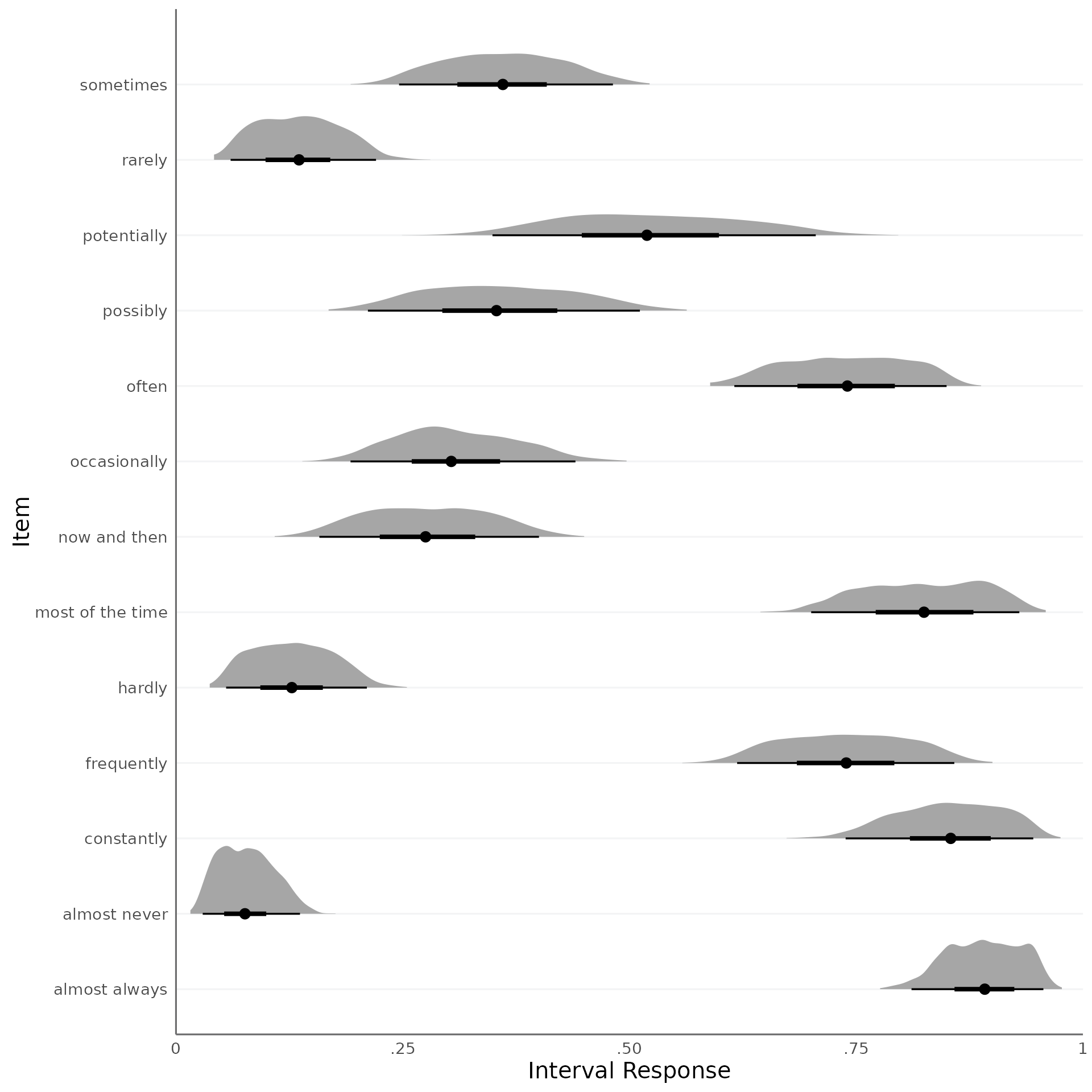
What does the dataset look like? We can visualize the interval responses using the plot_intervals_cumulative function:

plot_intervals_cumulative(
  lower = quantifiers$x_L,
  upper = quantifiers$x_U,
  min = quantifiers$scale_min,
  max = quantifiers$scale_max,
  cluster_id = quantifiers$name_en,
  weighted = TRUE
)
#> Warning: Removed 390000 rows containing missing values or values outside the scale range
#> (`geom_vline()`).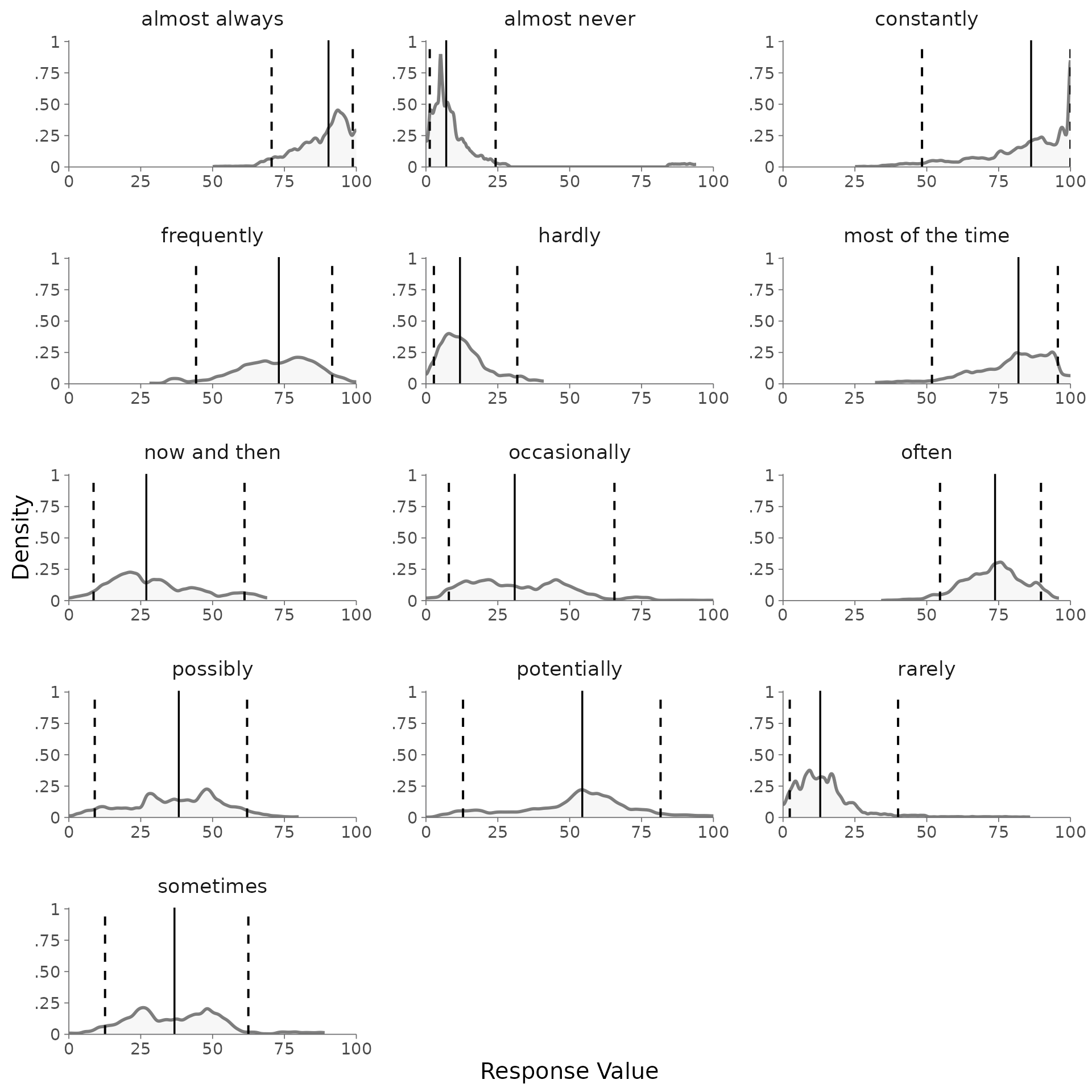

Next, we need to convert the interval responses to the simplex format:

quantifiers <- cbind(
  quantifiers, 
  itvl_to_splx(quantifiers[,c("x_L","x_U")], min = quantifiers$scale_min, max = quantifiers$scale_max))

head(quantifiers[,9:13]) |> 
  round(2) |>
  kable() |> 
  kable_styling()

x_L	x_U	x_1	x_2	x_3
31	65	0.31	0.34	0.35
27	61	0.27	0.34	0.39
66	80	0.66	0.14	0.20
11	28	0.11	0.17	0.72
40	47	0.40	0.07	0.53
60	70	0.60	0.10	0.30

Let’s check if we can apply the Isometric Log-Ratio transformation:

try(ilr(quantifiers[,c("x_1","x_2","x_3")]))
#> Error in check_simplex(simplex[i, ]) : 
#>   Error: None of the elements in the (row-)vector must be exactly 0! Please apply padding first!

It seems we have components in our simplex data that are zero. So we first have to deal with these zero components. We can do this by adding a padding constant:

quantifiers[, c("x_1", "x_2", "x_3")] <- 
  remove_zeros(quantifiers[, c("x_1", "x_2", "x_3")], padding = 0.01)

head(quantifiers[,9:13]) |> 
  round(2) |>
  kable() |> 
  kable_styling()

x_L	x_U	x_1	x_2	x_3
31	65	0.31	0.34	0.35
27	61	0.27	0.34	0.39
66	80	0.65	0.15	0.20
11	28	0.12	0.17	0.71
40	47	0.40	0.08	0.52
60	70	0.59	0.11	0.30

fit <-
  fit_itm(
    df_simplex = quantifiers[, c("x_1", "x_2", "x_3")],
    id_person = quantifiers$id_person,
    id_item = quantifiers$id_item,
    item_labels = quantifiers |> 
      dplyr::distinct(id_item, name_en) |> 
      dplyr::pull(name_en),
    n_chains = 2,
    n_cores = 2,
    iter_sampling = 1000,
    iter_warmup = 300,
    adapt_delta = .95
  )

Now we can extract the estimated cosensus intervals from the fit object. The function returns a list containing the posterior samples and a summary table of the consensus intervals stemming from the posterior medians.

consensus <- extract_consensus(fit, print_summary = FALSE)
attributes(consensus)
#> $names
#> [1] "df_rvar" "summary"

If we want to get a summary of the consensus intervals, we can use the summary function, which is a wrapper function around extract_consensus.

summary(fit) |>
  round(2) |> 
  kable() |> 
  kable_styling()

	T_L_median	T_L_CI_025	T_L_CI_975	T_U_median	T_U_CI_025	T_U_CI_975
now and then	0.17	0.12	0.23	0.38	0.32	0.45
possibly	0.23	0.17	0.30	0.48	0.40	0.57
almost always	0.83	0.78	0.87	0.96	0.93	0.97
almost never	0.03	0.02	0.05	0.12	0.09	0.16
occasionally	0.21	0.16	0.28	0.40	0.32	0.48
frequently	0.63	0.58	0.68	0.86	0.81	0.90
hardly	0.06	0.04	0.08	0.20	0.16	0.24
sometimes	0.26	0.21	0.32	0.46	0.39	0.52
most of the time	0.72	0.66	0.77	0.93	0.89	0.96
often	0.63	0.58	0.68	0.85	0.81	0.88
potentially	0.38	0.28	0.48	0.68	0.57	0.77
rarely	0.06	0.04	0.09	0.21	0.16	0.27
constantly	0.77	0.68	0.84	0.94	0.90	0.97

We can also plot the estimated consensus intervals. The generic function plot calls the function plot_consensus with the default method median_bounds.

plot(fit, method = "median_bounds")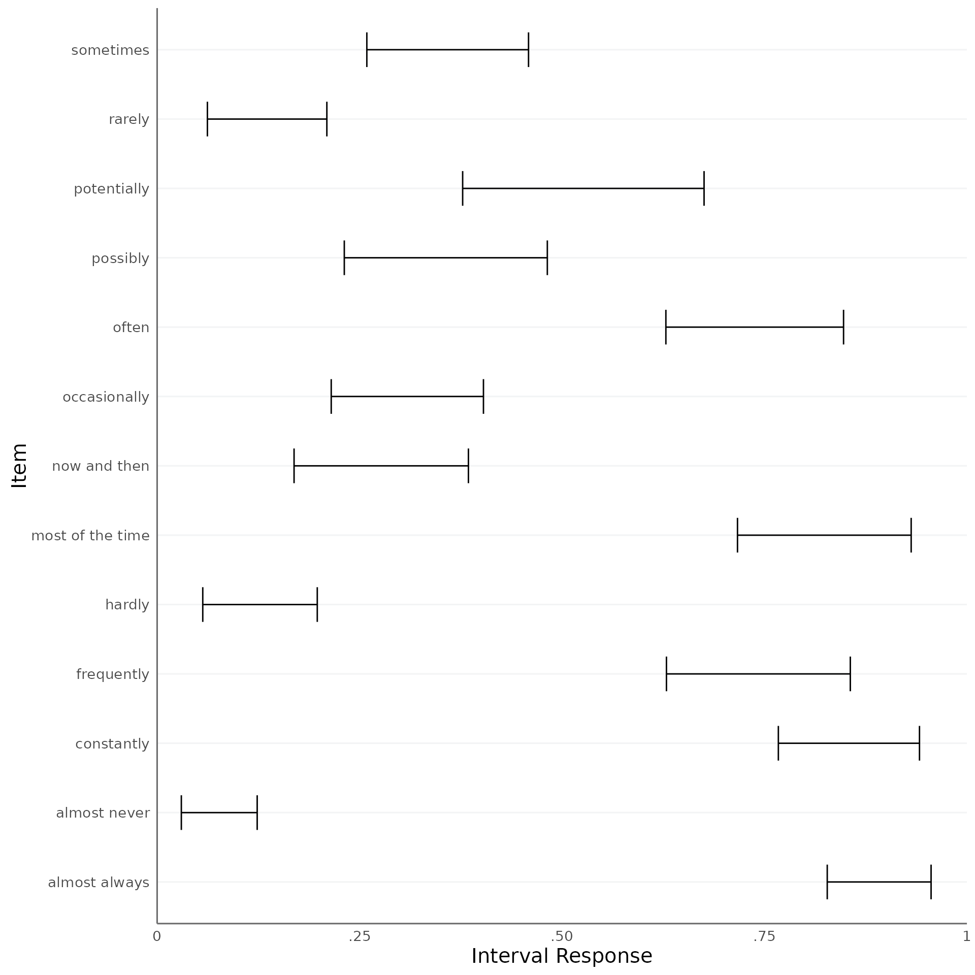

We can call the function plot_consensus directly for the alternative plotting method draws_gradient. This method plots the consensus intervals based on the posterior draws. For every posterior draw, a sample is drawn from a uniform distribution using the respective interval bounds of the posterior draw as minimum and maximum. The result is an rvar containing the values from the respective consensus interval, which is visualized in the plot.

An alternative method is draws_gradient which plots the consensus intervals based on the posterior draws. For every posterior draw, a sample is drawn from a uniform distribution using the respective interval bounds of the posterior draw as minimum and maximum. The result is an rvar containing the values from the respective consensus interval, which is visualized in the plot. The argument CI specifies the credible interval for this distribution and CI_gradient specifies the credible interval outside which the uncertainty is visualized by a gradient.

plot_consensus(fit, method = "draws_distribution", CI = .95)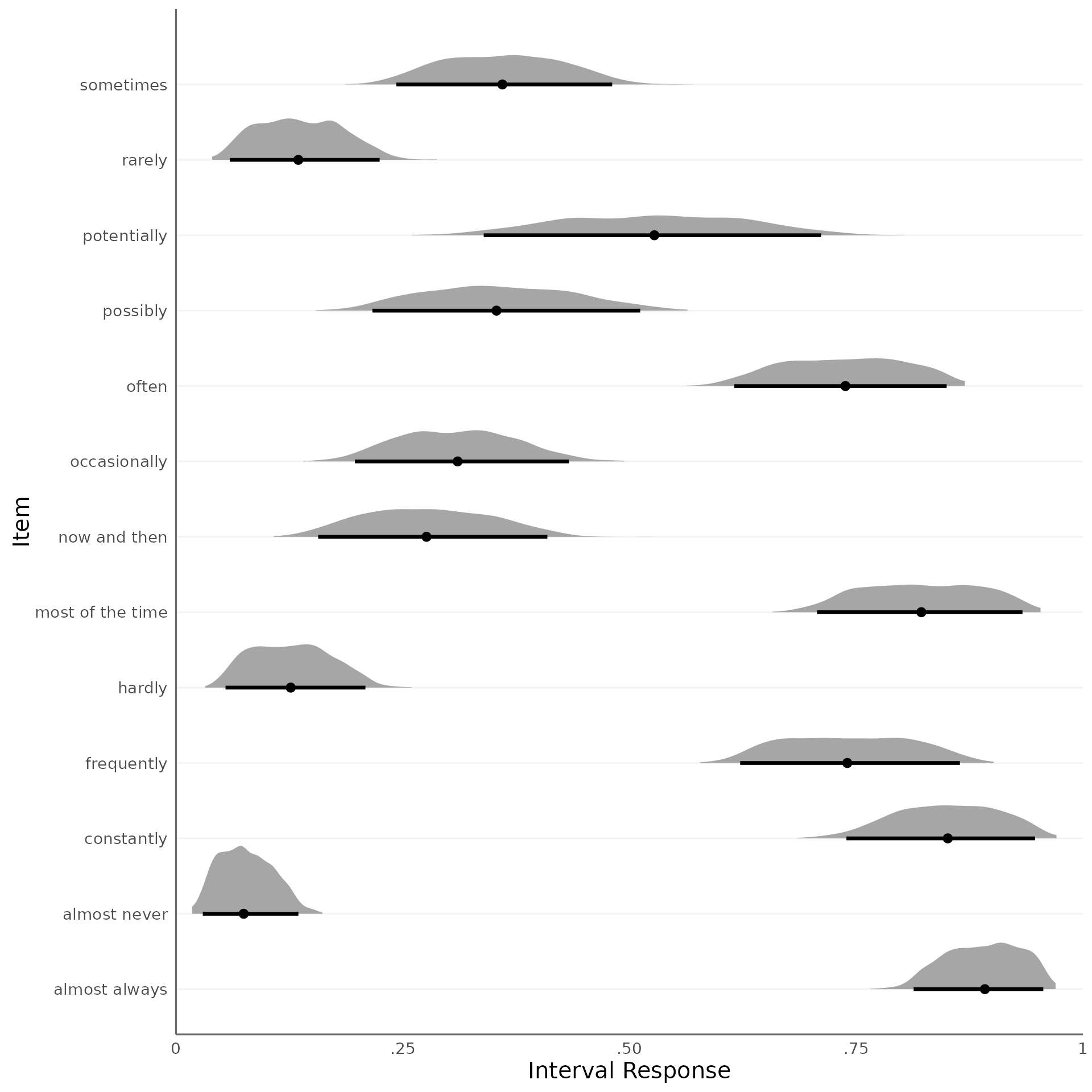

plot_consensus(fit, method = "draws_distribution", CI = c(.5,.95))